Hybrid Tracker

This work is published in IEEE Sensors, 2013 and IEEE Robotic and Sensors Environments (ROSE), 2013.

Tracking systems are essential components for many computer assisted interventions because they enable the doctor to visualize anatomical information, derived from preoperative or intraoperative images, registered with respect to the actual patient anatomy. This study presents two applications of Bayesian filters: Particle Filter (PF) and Extended Kalman Filter (EKF) to obtain accurate dynamic tracking performance from an electromagnetic tracking (EMT) system, even if the EMT cannot provide the full measurement state at each sampling interval (for example, when transmit coils are driven sequentially and/or receive coils are not sampled simultaneously). Experiments are performed with a custom EMT system, consisting of a transmitter coil array and one or more receiving coils, to demonstrate that the proposed method provides good dynamic tracking accuracy at different velocities.

For this project we have been developing a hybrid tracking approach, using EMT and inertial sensing, to create a tracking system that has high accuracy, no line-of-sight requirement, and minimal susceptibility to environmental effects such as nearby metal objects [1]. Our initial experiments utilized an off-the-shelf EMT and inertial measurement unit (IMU), but this introduced two severe limitations in our sensor fusion approach: (1) the EMT and IMU readings were not well synchronized, and (2) we only had access to the final results from each system (e.g., the position/orientation from the EMT) and thus could not consider sensor fusion of the raw signals. We therefore developed custom hardware to overcome these limitations. It is not trivial, however, to design an accurate EMT. One challenge is dynamic accuracy, which is the accuracy of the EMT measurements when the tracked object (which contains the receiving coil) is in motion. Nafis et al. [2] performed experiments to measure the dynamic tracking accuracy of several commercially-available EMTs. They found that many of these systems did, in fact, show significant increases in error as the velocity increased (e.g., see Fig. 19 in [2]), although some maintained good accuracy even at high velocities. However, because these are proprietary systems, the details of their design are not known.

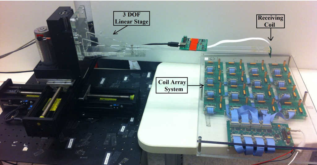
Our custom tracking system was developed by the Fraunhofer Institute for Manufacturing Engineering and Automation (Fraunhofer IPA) as part of a joint research project to investigate a hybrid tracking approach [1]. This hybrid tracker integrates electromagnetic and inertial sensing and provides synchronized readings at a 1 kHz sampling rate (Fig. on the left). For the methods and experiments reported in this paper, we use only the EMT component of this system. The EMT is composed of two parts: (1) an array of transmitting coils, and (2) a receiving coil (the design supports up to 3 orthogonal receiving coils, but we are using just one). The transmitter array has a 4 x 4 array of x-, y-, and z-direction coils, for a total of 48 coils. The coils are 23 mm in length and are arranged 75 mm apart from one another. In this study, only the perpendicular (z-direction) coils are used for tracking purposes, similar to [3]. At each instant of time, one of the coils is excited with a square wave signal and the induced voltage is measured from the receiving coil. This voltage does not appear immediately because it takes some time for the transient voltage to diminish and reach steady state. This transition period, which determines the update rate of our system, can be seen below.

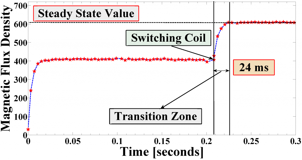
In the plot above, the red stars represent the measured voltage, which corresponds to the dipole field strength. As can be seen, after switching one coil, it takes approximately 24 ms for the readings to settle down and this determines the maximum update rate of our EMT system (41.67 Hz).

Bayesian Filtering

Recursive filters, such as particle filters and Kalman filters, are well suited for cases where data is obtained sequentially, rather than simultaneously [6]. These filters have a prediction stage and an update stage. In the prediction stage, the system model, is used to estimate the state vector, between each measurement. Then, in the update stage, the goal is to modify the state predictions using the latest measurement.

To describe the near field seen by a receiving coil, the dipole field approximation is used (e.g., in [3], [4] and [5]). This model also forms the measurement model of the Bayesian filtering model. For the system model, on the other hand, a constant velocity model is used.

Particle Filtering Implementation: In this filtering technique, the goal is to accurately predict the state probability density function (pdf) between each measurement. To accomplish this, a predetermined number of solution candidates (particles) are randomly created in the solution space defined by the process model. Next, depending on the closeness of the measurement model equation, a weight is given to each particle. The solution becomes the superposition of the solution candidates (particles) with respect to these weights. For the implementation of particle filters there are various methods, such as: Sequential Importance Sampling (SIS), Sampling Importance Resampling (SIR), and Regularized Particle Filter (RPF). We implemented SIR with systematic resampling.

Extended Kalman Filter Implementation: Similar to PF, Kalman filtering is a well known Bayesian Filtering technique and it is used in many other tracking applications. The Kalman filter is an optimal estimator if the system and measurement models are linear and the noises have Gaussian distributions. However, for the EM tracking problem, the measurement model is nonlinear so it is necessary to use an extended Kalman filter, where the measurement model is linearized with respect to the state variables.

We used a motorized linear stage (one axis of a 3-axis Cartesian robot) to test the dynamic tracking accuracy of our custom EMT. We used just a single axis of the robot to ensure linear motion. To eliminate field distortions due to nearby metal objects, we attached the receiving coil to the tip of a Plexiglass beam. We moved the linear stage at various velocities, while measuring the receiving coil voltage and estimating its position and orientation.

For the experiments, we placed the Cartesian robot at an orientation that was not aligned with any axis of the EMT. We moved the linear axis 20 cm and used the same trajectory pattern starting from different locations in the EMT measurement volume. We defined the ground truth trajectory to be the best-fit line to the tracking data that we estimated for both PF and EKF methods at all velocities. Additionally, we defined the error as the minimum distance between a calculated point and the ground truth line in three dimensions.

* LM solution (no motion compensation) For static EM tracking, the LM method is a well suited option[3]. However, it performs poorly under dynamic tracking, which reveals the need for another method for tracking moving objects. To better analyze how the LM method performs for dynamic target tracking, we generated synthetic data for receiver coil measurements at a known trajectory at different velocities similar to the experimental setup. We generated two sets of data: 1) without any measurement noise, and 2) with measurement noise N(0,σ^2) (Figure below on the left).

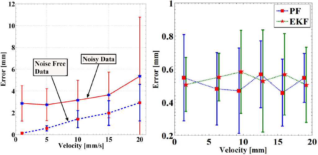
* Extended Kalman Filter (EKF) and Particle Filter (PF) Solution

We used real experimental data to test the EKF and PF because the synthetic data produced nearly perfect results (not surprising, considering that the synthetic data had no noise, or a perfectly known noise model). Specifically, we used a single axis of the robot system to obtain rectilinear motion of the receiver coil, as explained in Section IV. We moved the linear stage at 1.5 mm/s, 6 mm/s, 9.5 mm/s, 13 mm/s, 16 mm/s and 19 mm/s. Figure on the upper right shows the position errors for all velocities with PF and EKF. The error is reduced to sub-millimeters with the Bayesian filtering approaches. Furthermore, the shows that the mean position error remains relatively constant even when the velocity increases. The lowest standard deviation of the error is produced by the EKF at low velocities and by the PF at high velocities.

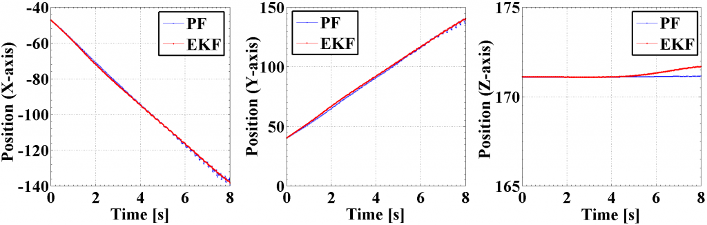
Figure above also shows the estimated trajectory over time at V = 16 mm/s. In these plots it is seen that the target motion is linear in both the x and y axis directions and stays nearly constant in the z axis direction. Both methods yield similar performance, with the PF exhibiting small oscillations in the x and y directions and the EKF showing slightly larger deviations in the z direction (investigation of these minor anomalies is the subject of future work).

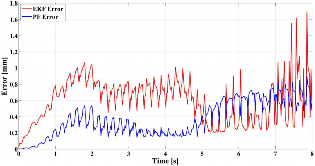
The figure above shows the position error versus time under the same conditions. Here, the position error is defined as the magnitude of the minimum length vector between the estimated position and the best-fit line computed from all data sets. Both methods achieve a mean error of approximately 0.55 mm, with the PF showing less variance about the mean. Although the experiments so far have focused on position tracking, PF and EKF also estimate the 2D angular orientation of the coil, thus providing a 5 DOF result.

[1] H. Ren, D. Rank, M. Merdes, J. Stallkamp, and P. Kazanzides, “Development of a wireless hybrid navigation system for laparoscopic surgery,” in Medicine Meets Virtual Reality 18, pp. 479–485, 2011.

[2] C. Nafis, V. Jensen, L. Beauregard, and P. Anderson, “Method for estimating dynamic EM tracking accuracy of surgical navigation tools,” in Proc. SPIE Medical Imaging: Visualization, Image Guided Procedures, and Display, vol. 6141, Mar 2006.

[3] A. Plotkin and E. Paperno, “3-D magnetic tracking of a single subminiature coil with a large 2-D array of uniaxial transmitters,” IEEE Trans. Magnetics, vol. 39, pp. 3295–3297, Sep 2003.

[4] M. Li, S. Song, C. Hu, and M. Q.-H. Meng, “A novel method of 6-dof electromagnetic navigation system for surgical robot,” World Congress on Intelligent Control and Automation, pp. 2163–2167, 2010.

[5] C. Hu, M. Li, S. Song, W. Yang, R. Zhang, and M. Q.-H. Meng, “A cubic 3-axis magnetic sensor array for wirelessly tracking magnet position and orientation,” IEEE Sensors, vol. 10, pp. 903–913, May 2010.